|
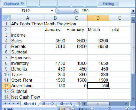
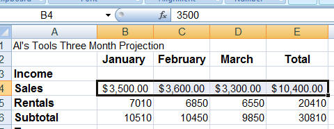
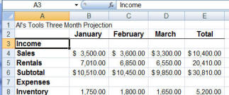
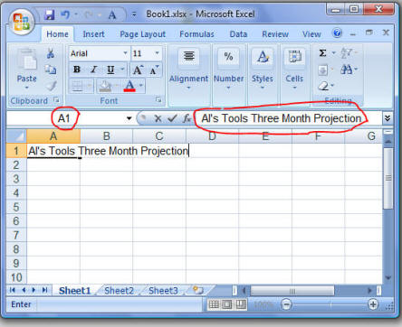
Enter the number data as shown.
|

|
-
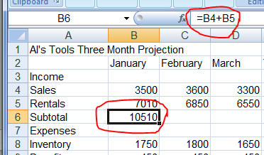
Next you will enter a formula in cell B6 that will add the values
of cells B4 and B5 together. Note: All formulas start
with the '=' sign.
-
Select cell B6.
-
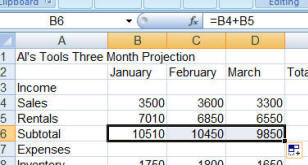
Enter the formula =B4+B5
-
Press the <Enter> key.
-
Again select cell B6
-
Notice that the value of cell B4 (3500) and the value of cell
B5 (7010) have been added together (10510) and placed
in cell B6.
-
Also notice that the formula box displays the formula you
entered in cell B6, not the value.
|

|
-
Cells C6 and D6 need a similar formula and you could enter =C4+C5
and =D4+D5, respectively. Or you could use the
fill method to automatically build the new formulas from the
formula in the adjacent cell as follows:
-
Select cell B6 so that it is ringed with a dark
border that has a small black square on the lower right edge of the cell
-
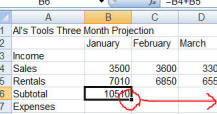
Click and drag the small square handle to the right so that cells C6
and D6 are highlighted
-
release the mouse button.
-
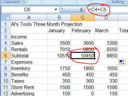
Notice that cells C6 and D6 have the correct values.
-
Select cell C6 to verify that it contains the formula
=C4+C5.
-
Notice that Excel has filled the formula from cell B6 to cells C6 and D6 while
changing the 'relative' addresses from B4 and B5 in the original formula
to C4 and C5, etc.
|


|
For Total Column (cell E4 for example) we could just enter the same addition
type formulas (=B4+C4+D4) as we did for the Subtotal row. Or we could use
Excel's SUM function as follows:
-
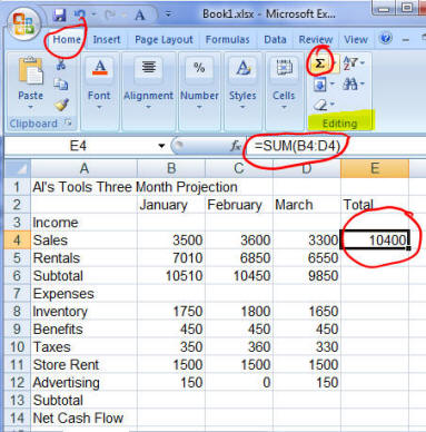
Select cell E4
-
Double-click the Sum button in the Editing area tool box on the Home
tab of the Ribbon.
-
Notice the correct value is displayed in cell E4, while the
Formula Box shows the Sum function =SUM(B4:D4)
-
The argument inside of the parentheses B4:D4
indicates the range of cells that are to be added
together (in this case cells B4, C4 and D4). Any cells between the
first cell listed and the cell listed after the ':'
are included in the summing function.
|

|
|
Use the fill method to place
the correct relative formulas in cells E5 and E6.
|

|
|
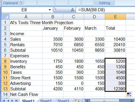
Then, use the Sum function and fill
method presented above to place the correct formulas in the
Expenses Subtotal row (cells B13 through D13), as well as the
Total Column (cells E4 through E6 and E8 through E13).
|
|
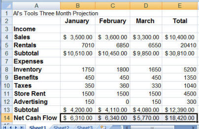
The Net Cash Flow row will calculate the difference between Income Subtotals
and Expenses Subtotals.Enter the =B6-B13 in cell B14 and fill
the formula through cells C14, D14, and E14.
The worksheet is now ready for formatting! Now would be a good time to save the
workbook as well. Save it as Excel Tutorial on your student data disk.
|

|
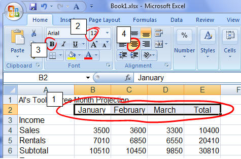
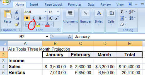
Start by making the Column headings 12 point, bold and aligned center:
-
Select the range B2 through E2 by clicking the
center of cell B2 and drag the mouse to the
right until all the cells are highlighted
-
Use the Font drop list in the to change the point size to
'12'
-
Click the bold button
-
Click the align center button
|

|
-
Apply the same technique to make the Row headings 12 point
and bold, but leave the alignment as it is (the default left aligned)
-
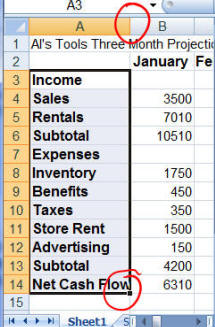
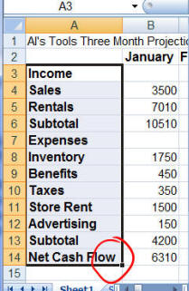
Note: Column A may not be wide enough to hold 'Net Cash Flow'
-
If that is the case, simply place the cursor on the border
between Column A and Column B as you did before and drag
the border to the right until there is enough room for 'Net Cash
Flow' label to fit
|


|
Formatting numbers is next.
-
The top row, Subtotal rows and Net Cash Flow row will have dollar signs,
commas and a decimal
-
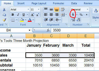
Select the range B4 through E4
-
Click the Accounting Number Format button ($)
-
Notice the cells now have dollar signs, commas and a decimal point
-
Also note that the widths of Columns B, C, D and E were automatically
expanded to handle the additional symbols
-
Note: If you see ####### instead of the expected
formatted number in a cell, it means the Column width needs to be
increased
|


|
|
Use the same technique to apply Accounting Number Format to the Subtotal
rows and the Net Cash Flow row
|

|
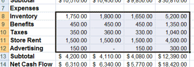
The other numbers will need commas and decimals to look correct.
-
Select the range B5 though E5,
-
click the Comma Style button (,)
-
Do the same with the range B8 though E12.
|


|
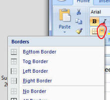
Using a border on certain cells can improve the readability of the worksheet.
-
Select the month labels in Row 2
-
Click the drop list arrow to expose the Borders menu
-
Click the Bottom Boarder button
-
Click cell A3 to move away from the Months labels and
see the formatted cells with a bottom border.
|


|
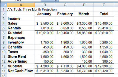
|
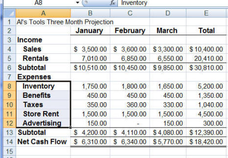
Apply the same technique to format the borders as shown.
Note: The Net Cash Flow row uses the Top and Double
Bottom Border
|

|
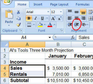
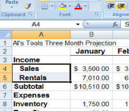
The row labels in Column A can be improved by indenting the subheadings under Income and Expense.
-
Select cells A4 and A5
-
Click the Increase Indent button to move the two labels to the right.
-
Apply the same technique to indent the Expenses subheadings.
|


|
The last step is to make the Report title larger and centered on the worksheet cells.
-
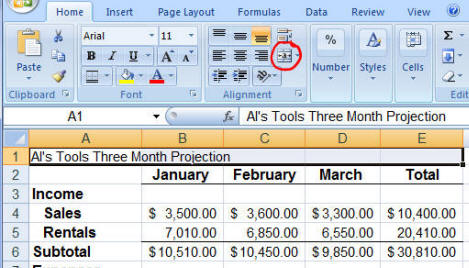
Select cells A1 through E1
-
click the Merge & Center button to merge the five cells into
one and center the Report title.
-
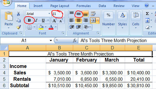
Then click the specific formatting buttons to make the Report
title 16 point, bold and vertical aligned center.
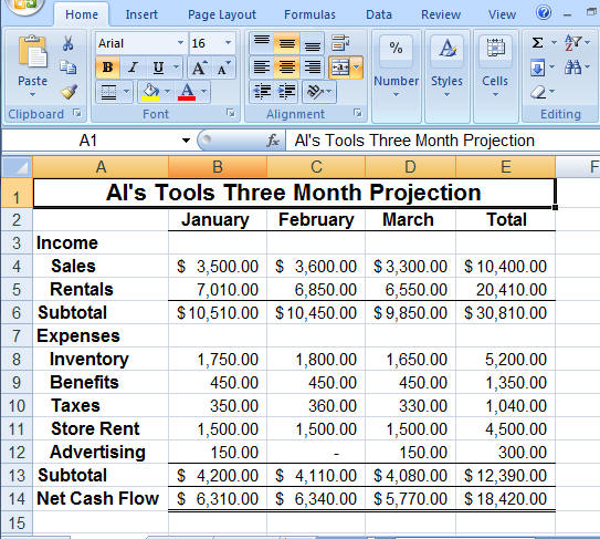
And there you have it... the completed spreadsheet for Al's Tools
Three Month Projection!
-
Save the document, naming it Al's Tools Three Month Projection.xlsx
|


|
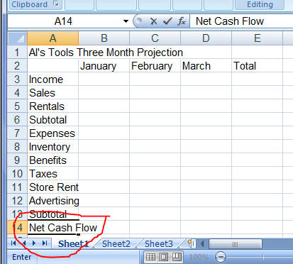
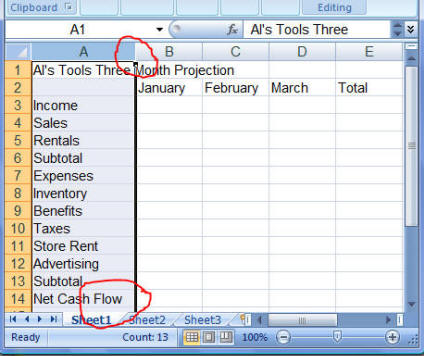
 and drag it to the right until Net Cash Flow is entirely
in cell A14.
